Treasure Trails, Part 2

This is the second of two posts. In this one I’m just doing math, but if you want to see what I’m talking about, you’ll want the first part.

When designing something like treasure trails, I start to ask myself questions about how it behaves. How long is the shortest/longest/average trail? Is “intel” a more likely reward than “loot”? What is the size of the average loot hoard? How quickly will a riddle be repeated? How many trails will it take to “finish” the conspiracy? What types of clue are more or less common? And so on. Questions like these grow to eat my free moments until I exorcise them.

Exact Solutions

The system as outlined (roll 1d6+n, where n is the number of preceding rolls, stop on a result of 7+), can be modeled as an absorbing Markov process, like Snakes & Ladders. The states of our process are $n=0$, $n=1$, $n=2$, …, $n=6$, and “finished.”

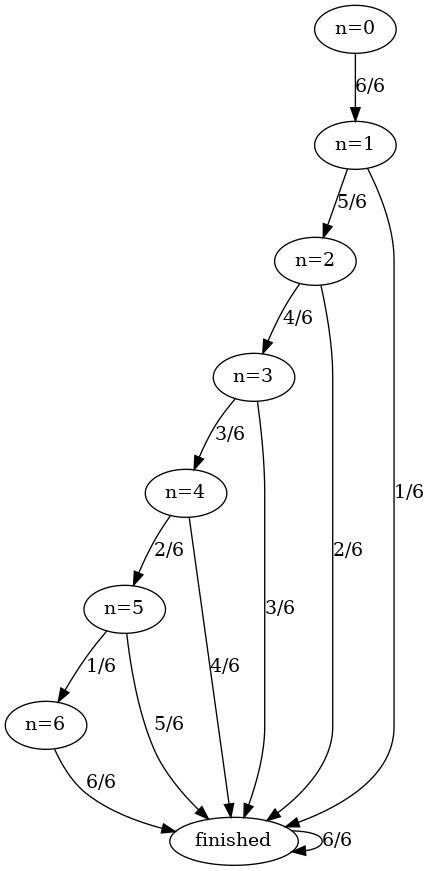A graphical representation of the possible states of our system.

From this, we can construct a transition matrix,

${\displaystyle P=\left[\begin{array}{cccccccc}0& 6\mathrm{/}6& 0& 0& 0& 0& 0& 0\\ 0& 0& 5\mathrm{/}6& 0& 0& 0& 0& 1\mathrm{/}6\\ 0& 0& 0& 4\mathrm{/}6& 0& 0& 0& 2\mathrm{/}6\\ 0& 0& 0& 0& 3\mathrm{/}6& 0& 0& 3\mathrm{/}6\\ 0& 0& 0& 0& 0& 2\mathrm{/}6& 0& 4\mathrm{/}6\\ 0& 0& 0& 0& 0& 0& 1\mathrm{/}6& 5\mathrm{/}6\\ 0& 0& 0& 0& 0& 0& 0& 6\mathrm{/}6\\ 0& 0& 0& 0& 0& 0& 0& 1\end{array}\right]}$

It works like this: if you are on step “$n=2$,” you multiply by a column with only that row filled:

${\displaystyle \left[\begin{array}{cccccccc}0& 6\mathrm{/}6& 0& 0& 0& 0& 0& 0\\ 0& 0& 5\mathrm{/}6& 0& 0& 0& 0& 1\mathrm{/}6\\ 0& 0& 0& 4\mathrm{/}6& 0& 0& 0& 2\mathrm{/}6\\ 0& 0& 0& 0& 3\mathrm{/}6& 0& 0& 3\mathrm{/}6\\ 0& 0& 0& 0& 0& 2\mathrm{/}6& 0& 4\mathrm{/}6\\ 0& 0& 0& 0& 0& 0& 1\mathrm{/}6& 5\mathrm{/}6\\ 0& 0& 0& 0& 0& 0& 0& 6\mathrm{/}6\\ 0& 0& 0& 0& 0& 0& 0& 1\end{array}\right]\times \left[\begin{array}{c}0\\ 0\\ 1\\ 0\\ 0\\ 0\\ 0\\ 0\end{array}\right]=\left[\begin{array}{cccccccc}0& 0& 0& 4\mathrm{/}6& 0& 0& 0& 2\mathrm{/}6\end{array}\right]}$

The resulting vector shows the probability of the next state, here “$n=3$” with probability 4/6 and “finished” with probability 2/6. More complex systems can be imagined here! We could introduce a type of clue that counts twice, or doesn’t count at all. We could even change the size of the die as we go.

If multiplying an input state by $P$ produces the distribution of output states after one step, multiplying by $P^2$ produces the distribution of output states after two steps. Multiplying by $P + P^2$ gives us the odds of visiting a given state in either of the two steps. If we sum

${\displaystyle \sum _{k=0}^{\mathrm{\infty }}{P}^k}$

Then this will give us the probability of visiting any given state throughout the whole process. However, we actually want to use the sub matrix of $P$, $Q$, which only includes the transient states. (The “finished” state is the opposite, an absorbing state.) From $Q$, we can derive the fundamental matrix,

${\displaystyle N=\sum _{k=0}^{\mathrm{\infty }}{Q}^k={(I-Q)}^{-1}}$

where $I$ is the identity matrix.

The expected number of steps before being absorbed from a given state is the corresponding element of $t$ in

${\displaystyle t=N\times \mathbf{\text{1}}}$

where $\mathbf{\text{1}}$ is a column vector of all ones.

Rearranging, this gives us:

${\displaystyle \mathbf{\text{1}}=N^{-1}\times t=(I-Q)\times t=\left[\begin{array}{ccccccc}1& -6\mathrm{/}6& 0& 0& 0& 0& 0\\ 0& 1& -5\mathrm{/}6& 0& 0& 0& 0\\ 0& 0& 1& -4\mathrm{/}6& 0& 0& 0\\ 0& 0& 0& 1& -3\mathrm{/}6& 0& 0\\ 0& 0& 0& 0& 1& -2\mathrm{/}6& 0\\ 0& 0& 0& 0& 0& 1& -1\mathrm{/}6\\ 0& 0& 0& 0& 0& 0& 1\end{array}\right]\times \left[\begin{array}{c}{t}_0\\ t_1\\ t_2\\ t_3\\ t_4\\ t_5\\ t_6\end{array}\right]}$

which can be solved as a system of equations, and gives us $t_0$ clues as the average length of a treasure trail.

Less Exact Solutions

Whew, it’s been a long time since I learned linear algebra. And what if I want to ask a lot of questions, or tweak some parameters and ask again? Well, I’ve always wanted an excuse to play with Monte Carlo simulations.

So I wrote a little python script. From this we can see that the average trail length is ~2.77¹, which agrees with the theoretical solution above (the difference of 1 is whether or not the “reward” step is counted). We can see that intel (result 7) is slightly less common than loot (results 8+). The average loot roll is ~8.6 (although the average hoard size will depend on our mapping). The most common clue type is 6 (anagram) and the least common is 1 (compromised handoff). In fact, we can see that the frequency each clue type increases monotonically. We can even put together a pretty chart combining clue frequencies and rewards, which is a decent visual summary of the system.

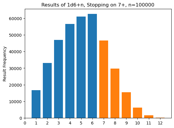A bar chart of result frequencies. Blue bars are clue types and orange bars are reward types.

From this, we can gain some insight. Putting the most difficult clue types at the start of our list will make longer trails more likely to have “easier” clues in them, which gives us a rough division between “short, difficult” and “long, easy” trails. But it also means that long trails get easier as they go, which could be unsatisfying. To stretch variety as long as possible, clue types that repeat less could be swapped into the more commonly rolled numbers. For example, handoffs (result 5) could swap with anagrams (result 6) because both are relatively straightforward, but there are many more variants of handoff than anagram.

Armed with this program, we can explore similar mechanics, rolling different dice and stopping at different numbers.

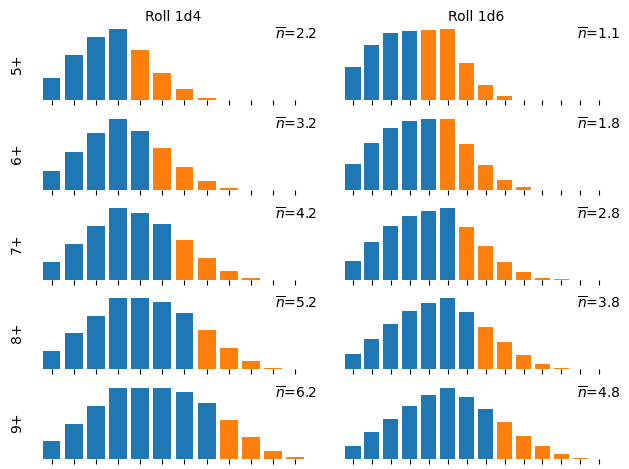An array of bar charts of result frequencies for different mechanics.

(In the above chart, ${n}$ is the average trail length, excluding the “reward” step.)

---

1. Especially with smaller values of $n$, this exact value may vary from run to run.↩︎

---

---

---

---

---

---