Combining Dice and Other Rules

In my review of Rod, Reel, & Fist (RRF), I mentioned that the distinction between two possible interpretations of the rules was largely unnecessary:

Worse, if a player or playgroup thinks that you can combine dice in a pyramidal fashion, let them! It hardly makes a difference, mathematically, as the comparison to a target number ultimately “smooths” out the advantage for all but the largest pools against the largest target numbers. (Rod, Reel, & Fist (Review), me)

I thought I’d take some time with these two mechanics, and some others, to more fully understand what makes the game tick.

RRF Mechanics

There are two relevant mechanics in this analysis: combining dice and fish combat. (Animal combat can be considered a variation of fish combat.)

Combining Dice

The general resolution mechanic in RRF is to roll one or more six-sided dice and attempt to meet or exceed a target number (TN) from 3 to 7 with at least one of the dice.

The smallest TN is 3, but 7 is only the largest base TN.¹ TN increases by one for each point of stress or exhaustion accumulated, with no upper bound.

If multiples are thrown, then the number of dice in the matching set is added to that die’s value. For example: ⚃⚃ → 4+2 → 6. This is the only way to beat a challenge with TN≥7.

The smallest pool size is 1; you cannot lose your last die. The largest pool size that matters is 16; any more than this will always succeed, even against TN=7 (although not TN>7).²

Examples

• ⚁⚁⚁ → 2+3 → 5
• ⚂⚂⚃ → 2+3, 4 → 5, 4 → 5
• ⚂⚂⚅ → 2+3, 6 → 5, 6 → 6
• ⚄⚃⚃⚁⚁ → 5, 2+4, 2+2 → 6

Fish Combat

Fish combat is the general procedure by which Fishers catch fish. The specifics of fish combat (and other combat) aren’t super important here, except for two points:

• Combat only ends when one party can fail a TN=3 “Hang On” test (made with stress and exhaustion, of course).
• Each participant has the opportunity to “strain” dice: removing a die from their own pool to remove a corresponding die from their opponent’s. You can neither strain, nor have strained away your last die.

Exploration

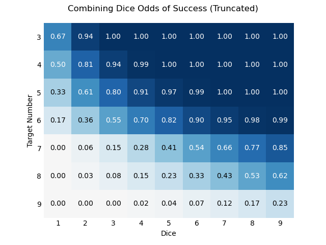
I wrote a script in Python to calculate the odds of succeeding a test, given a TN, a pool size, and a rule for evaluating the roll. The results can be shown on a heatmap.

A white square indicates no chance of success and a blue square indicates sure success.

Note that even though I extended the map out to 17 dice, the odds are effectively a sure thing much earlier. As we look at other mechanics, I’ve chosen to only display the first nine pools, where more interesting features can be seen clearly.

Pyramid Dice

Rather than repeat the section in RRF describing how this doesn’t work, I’ll rephrase it here as though it did:

Similarly, you [can] build pyramids out of your numbers. If you roll two 2s and one 4, those 2s Combine to become a 4, but they […] Combine again with the other 4 you’d rolled to become a 6. (Rod, Reel, & Fist, p. 32, significantly modified)

For example:

• ⚄⚃⚃⚁⚁ → 5, 4, 4, 2+2 → 5, 4, 4, 4 → 5, 4+3 → 5, 7 → 7

If we suppose that these were the rules for RRF, what would the heatmap look like?

This looks very similar to the naked eye.

We can also look only at the difference:

The numbers here represent the increased odds, relative to Combining Dice, and are shaded on the same scale as the other heatmaps.

What’s happening here? With only two dice, the odds are obviously identical to the built-in mechanic. But even with three dice, the odds of our new rule becoming relevant are still small: you need to roll doubles and then a “matching” number. The rule barely has any effect until you reach much larger dice pools.

At the same time, it doesn’t matter nearly as much at lower target numbers. This is because the actual value of the roll isn’t important, only whether or not it meets the target number. If I roll ⚁⚁⚃ against TN=4, it doesn’t matter that I can construct a 6 out of my numbers, I pass the test either way.

So the only place the new rule makes a real difference is at high target numbers with large dice pools.

Maximum Dice

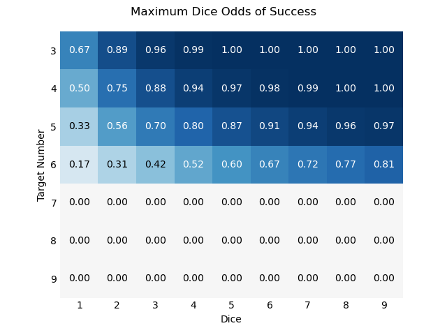
RRF explains Combining Dice as a means to reach TN=7, which is true, but might undersell its impact. Simply taking the maximum roll with no other math seems like a reasonable baseline for comparison.

For example:

• ⚄⚃⚃⚁⚁ → 5, 4, 4, 2, 2 → 5

These numbers are also relative to Combining Dice. Negative numbers show a decrease in odds of success, and are shaded red.

There are some interesting features to this. You can never make TN≥7, no matter how many dice you roll, so those rows are always “saturated.” Conversely, you can never fully be sure of success at TN≤6 no matter how many dice you roll. Rolling one more die is always better than not.

This rule is fascinating to me as a kind of “building block” of a mechanic, but it lacks a certain excitement and has a necessarily limited scale.

Sum Duplicates

A more common mechanic, we simply sum duplicate rolls before taking the maximum. Obviously this can generate much larger numbers than Combining Dice, but given how we saw target numbers limit the effects of the pyramid rule, we might expect something similar here.

For example:

• ⚄⚃⚃⚁⚁ → 5, 4+4, 2+2 → 5, 8, 4 → 8

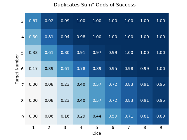
One interesting feature of this rule is that prime numbers, like seven, can’t be produced. So every prime TN > 6 will be just as difficult to reach as that TN+1 (as we see here with TN=8).

Negative numbers here are shaded red while positive numbers are blue, but it's hard to see as the decreases in odds are very small.

Compared to combining dice, this rule is also not uniformly more or less likely to succeed. Any sum of ones is actually one less than the value produced by RRF-style combining dice. Especially at low TNs, where successes are mostly successful under either rule, we can see this minuscule decrease in odds. But, as expected, there is a similar increase for larger dice pools at higher TNs, similar to the Pyramid rule.

Add One for Duplicates

A simpler-to-explain mechanic than Combining Dice (to my mind, at least), is that additional dice add one to the first copy. This necessarily gives smaller numbers than Combining Dice.

For example:

• ⚁⚁⚁ → 2+1+1 → 4
• ⚄⚃⚃⚁⚁ → 5, 4+1, 2+1 → 5, 5, 3 → 5

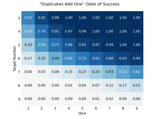
I don’t have much to say about this rule, as it’s very similar to the RRF Combining Dice rule already.

Metrics

If your eyes start to glaze over in this section, feel free to skip to the conclusions. If your eyes start to narrow in fury, please leave a comment telling me how I did it wrong!

Intuitiveness

There are two reasons combining dice works at all. First, adding a die to your die pool never decreases your odds of success. Second, adding another die to your die pool never increases your odds of success more than the last one did. Mathematically, we can say that for a given TN, the function is monotonic increasing, and its first derivative is monotonic decreasing (ideally).³

The top graph here is analogous to the first figure in the post. The graph below it is an approximation of its first derivative, and the graph below that it's second. As before, blue squares are positive, red squares are negative, and lighter squares are closest to 0.

These properties are not particularly exotic, and we may not find a natural rule that does not have them, but they are worth checking. The intuitive behavior of the rule is what allows the bluffing and betting behavior of fish combat.

To illustrate, we can consider a rule such that rolling three dice always succeeds, regardless of TN. The surface may be more interesting, but we want to focus on the complexity elsewhere; “interesting” is not our goal here.

This example is contrived, perhaps, but hopefully illustrative.

While monotonicity is our goal, it may not be possible with every rule. To facilitate comparisons, we can instead take as metrics the minimum of the first derivative and the maximum of the second derivative. In our ideal function, these will both be zero.

Saturation

When you have three dice, TN=3 is irrelevant to you. You cannot fail such a roll. We say that the function is saturated there: the odds of beating TN=3 are as good as they’ll ever get, and the tactical utility of choosing TN=3, has been, in a sense, exhausted. Similarly, if you have only one die, you will never beat TN=7. This too is a kind of saturation. This can be another metric by which we compare these ideas. ⁴

At zero, the function is unsaturated. There are decisions to be made and no role is a sure thing. At one, the function is completely deterministic and you never need to actually roll dice.

We can call the proportion of saturated states the saturation.

Odds of Success

Finally, sometimes a roll is required outside of combat, for example to test a Fisher’s knowledge. From this we can derive the metric average odds of success. Experience has shown that a game is most fun when the odds of success are in a player’s favor. We could try to choose a target range for how much so, but instead I am going to trust the saturation metric to keep this one in check: higher odds are better, but if they are too high, we expect the function to saturate faster.

Weighting

Now that we’ve defined some metrics, we face another problem: what good is it to know that I have full tactical decision making across any number of dice, if I’m only usually rolling 1-3 dice at a time? And, as we compare mechanics, how can we determine when to stop evaluating them?

The answer is to weight smaller dice pools more heavily than larger ones in our metrics, even though this requires some judgment on our part. The scheme I’m most familiar with is exponential weighting, which effectively weights each pool size according to a geometric progression.⁵ Arbitrarily, I’m choosing r=½, which means that pool size p=1 makes up ½ of the value, pool size p=2 makes up ¼, and so on.⁶

The weights of the first nine dice pools.

Now for practical purposes I can extend the heatmap to some large number of dice pools, say up to p=17. Contributions from the remaining terms will be very small but if we assume that the metrics are saturated by the 16th die, then we can weight the 17th equal to the sum of the remaining terms.

Under this scheme, our metrics are:

• Min 1st Derivative
• Max 2nd Derivative
• Weighted Saturation
• Weighted Odds

Conclusions

First let’s look at all the metrics we just discussed.

sat	odds	1stmin	2ndmax	mechanic
0.16	0.49	0.00	0.04	Combining Dice
0.18	0.50	0.00	0.07	Pyramid Dice
0.20	0.45	0.00	0.00	Maximum Dice
0.13	0.50	0.00	0.06	Duplicates Sum
0.13	0.48	0.00	0.02	Duplicates Add
0.26	0.53	-0.72	0.89	Threes Win

Metrics evaluated over TN in [3,7] over pools in [1,17], geometrically weighted with r=0.5 (where appropriate).

Not considering our purposely bad rule (“Threes Win”), we can see that they all perform remarkably similarly. “Maximum Dice,” as the rule that all the others are constructed from, sets a baseline: it is the most saturated and has the worst odds of success, but it also behaves the most intuitively (judging by the derivatives). For that matter though, the derivative requirements don’t seem particularly effective at differentiating between rules, as they all behave in “reasonable” ways.

The only rule of those examined that I would consider in place of “Combining Dice” is “Duplicates Add.” To my mind it is simpler to explain, and while the baseline odds of success are ever-so-slightly worse, the saturation is ever-so-slightly better. I think “Pyramid Dice” is too difficult to explain, “Maximum Dice” is ineffective for RRF by itself, and “Duplicates Sum” is worth excluding for its unintuitive behavior at TN=7 and TN=8, even if that may not be immediately obvious in play.

After all that, even though it seemed odd to me initially, there’s really no need to change the dice mechanics of RRF. Combining Dice is perfectly reasonable and works well for the game’s purposes. And any change we do make, we should be sure it’s worth the trouble: most rules look very similar once you apply them across all possible dice pools and compare those to a target number.

Once again, the code is here. Python is still fine, and when it all works out it’s a joy, but increasingly I wish it had the implicit type handling of Perl. (I also wish they didn’t insist on the word “pythonic,” when the perfectly functional “idiomatic” is right there.)

Happy fishing!

WINTER STEELHEAD TROUT FISHING ON THE SKAGIT RIVER, Doug Wilson, Public Domain, via Wikimedia Commons.

---

1. There is one reference in the book to a “super legendary” difficulty, at TN=8, but not within the rules themselves.↩︎

2. The largest pool size that can be achieved within the rules provided is 14: 1 base die, +1 die from the Angler type, +1 die (to Stand Firm) from the Tricky temperament, +2 dice (in the first round) from Artisan Boilies, +1 die from a tacklebox, +3 dice (on a full moon) from the Wolfish Rod, +2 dice from snacks, +1 die (to a known fish) from the Fist of the Zoologist technique, +1 die from a bargain with Pops Bailey, +1 die from William Jahl’s music. I expect the usual pool size will generally be much lower. The largest pool size available to a fish is 7.↩︎

3. We really only care about the first two derivatives here: the first derivative is how we reason about adding or removing dice from our own pool, and the second derivative is how we reason about changes in our opponent’s dice pool at the same time as our own (i.e. straining dice). This is also why I’m only evaluating these derivatives in the “horizontal” (dice pool) direction, and only stepwise (as opposed to with e.g. a central approximation, which here, may actually be less representative).↩︎

4. And it is important to note that this is strictly for comparative purposes. To understand how the mechanic behaves, we may not feel that a 99% chance is much different from a 98% chance. Rather than draw an arbitrary line at say, 95%, I am assuming that the proportion of states near saturation is similar to the proportion of actually saturated states.↩︎

5. I chose not to weight target numbers (or to evaluate metrics across them) because even though they can change with stress and exhaustion, for the most part they are bounded and equally available. For the same reasons, even though TN=8 and TN=9 are shown in each figure, they have been excluded from the calculation of metrics, because we do expect them to be less common.↩︎

6. Normally I could optimize the value of this constant over historical data to minimize sensitivity to noise and lag. In this case that would be both nonsensical and counterproductive.↩︎

---

---

---

---

---